Tackling Home Credit Default Risk with Machine Learning using scikit-learn

Credit risk assessment is a crucial task for financial institutions, as it helps them to make informed decisions about lending money to individuals. In this context, machine learning has become increasingly important, as it can help automate the process of assessing the credit risk of individuals. Let's explore how I built a machine learning project (assigned to me by AnyoneAI) to predict loan default risk, using the Home Credit Default Risk Kaggle competition dataset. I will take you through my data exploration, feature engineering, model training, and optimization process. Additionally, I will show you how to put all the pieces together using pipelines to automate the whole process.
Data exploration
The first step in any machine learning project is to explore the data. First, we need to download two datasets, application_train_aai.csv and application_test_aai.csv, which contain the training and testing data, respectively. The training dataset contains 246,008 rows with 122 columns, and the testing dataset contains 61,503 rows.
We have one target column, "TARGET," which indicates whether the individual was able to repay their credit in time (TARGET=0) or not (TARGET=1). Note that this column is empty in the test dataset, which means the target values are hidden from us. Our job is to predict these target values, and submit the test dataset with the predictions.
Let’s see the distribution of this target variable.
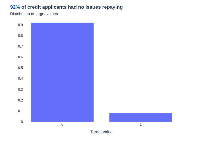
The target variable is unbalanced, with only around 8% of applicants having defaulted on their loans. This imbalance can lead to biased models that perform poorly on predicting the minority class. Therefore, it is important to take this imbalance into account when training our models.
Preprocessing and feature engineering
After exploring the data, the next step is to prepare the data for training ML models. I started by splitting the training data into training and validation datasets, in order to evaluate the models to be trained. In this step, I used a “stratify” parameter to so that the training and validation datasets have the same proportion of target values.
Having split the data, I performed the following transformations on the data.
- Encoding categorical variables: I used an OrdinalEncoder for variables with only two categories and a OneHotEncoder for variables with more categories.
- Filling in missing values: I employed a SimpleImputer with a "median" strategy to handle missing data.
- Scaling the data: I used a MinMaxScaler to scale the data, so that all features are in the same range.
The function in which I apply these transformations is a bit too long to show here. You can check it out in the project’s repo.
Model Training and evaluation
With the data preprocessed, I moved on to training machine learning models. First, I trained a LogisticRegression model as a baseline, achieving a validation ROC AUC Score of 0.68. Wait, what is the ROC AUC score?
The ROC AUC (Area Under the Receiver Operating Characteristic Curve) score is an evaluation metric for binary classification problems, as it measures the model's ability to distinguish between positive and negative classes. An ROC AUC score of 0.5 means that the model is as good as random, while a score of 1.0 means that the model is perfect.
Next, I experimented with a RandomForestClassifier, obtaining a training ROC AUC score of 1 and a validation ROC AUC of 0.71, which is slightly better than the baseline, but is a clear sign of overfitting.
To address this, I trained another random forest with class_weight="balanced" using RandomizedSearchCV, in order to find the best possible combination of hyperparameters for the random forest.
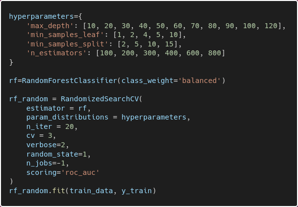
This yielded a training ROC AUC of 0.99 and a validation ROC AUC of 0.74. It is still overfitting, but is an acceptable validation score per the project’s requirements.
To further improve the results, I trained a LightGBM model, achieving a training ROC AUC of 0.8 and a validation ROC AUC of 0.76, which demonstrated better performance with much less overfitting. However, I did not run predictions on the test dataset using this model because the project requirement is to use Random Forest to predict on test data.
Putting it all together with pipelines
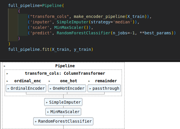
To automate the entire process of encoding, imputing, scaling, and training the RandomForestClassifier, I used sklearn Pipelines and ColumnTransformer. Pipelines are a powerful tool that allow us to string together multiple processing steps and models into a single object. The ColumnTransformer allows us to apply different preprocessing steps to different columns of our data. This results in a cleaner and more efficient workflow, making it easier to manage transformations and model training.
This is the code for the final pipeline.
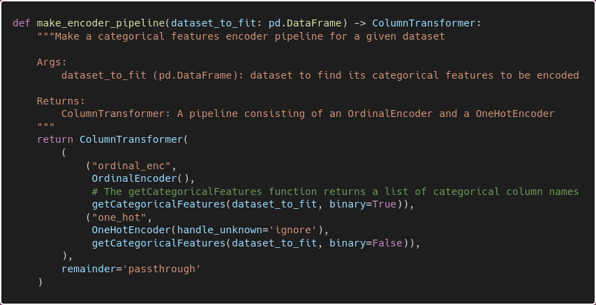
And the code for the make_encoder_pipeline function, which uses ColumnTransformer to execute the OrdinalEncoder and the OneHotEncoder in parallel.
Conclusion
We explored how to use machine learning to predict credit default risk using the Home Credit Default Risk Kaggle competition dataset. I showed you how I performed data exploration, feature engineering, model training, and optimization. I also introduced the concept of pipelines and showed how they can be used to automate the entire process. Thank you for reading, and stay tuned for my next machine learning posts.